Discrete Decisions, Fuzzy Mathematics Part 1

Updated after publication: Raised the grid coordinate bound to 2^61; the original bound was more conservative than needed to avoid overflow.

I’ve recently been fixing numerical edge cases in cavalier_contours in which calculations disagree with what the geometry tells us must happen. At the root of all these issues is the gap between mathematical (algebraic or topological) reasoning and numeric computation.

For example, consider two segments joined at a shared endpoint and a third segment that passes through that point:

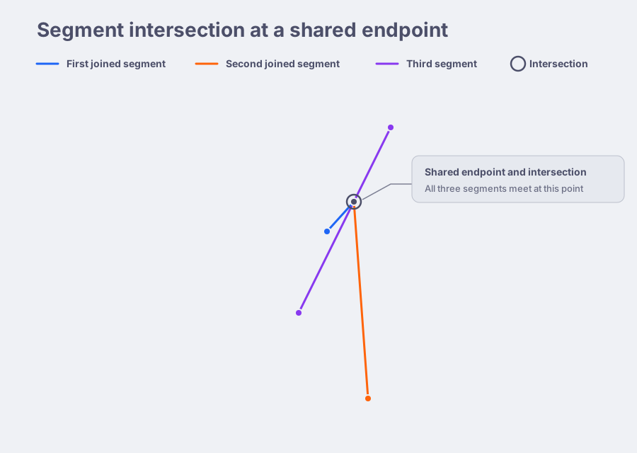
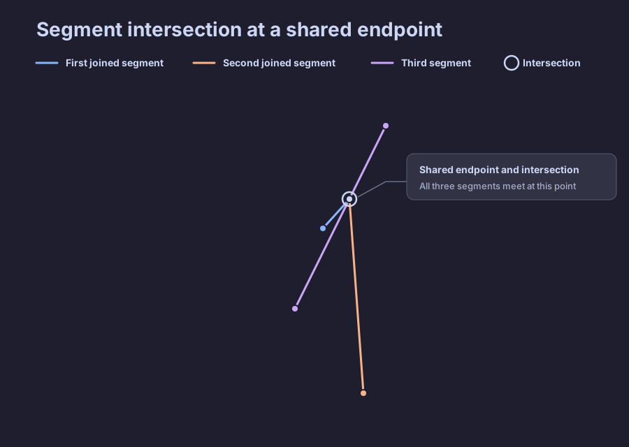
All three segments intersect at that point by definition, yet a floating-point calculation using the correct mathematical formula can still miss the intersection. How can that happen?

This will be the first post in a series intended as a dense tour¹ of this problem space. In this series, I’ll be covering:

• Numeric computation: what are we dealing with?
• A simple example in which numeric computation produces a mathematically impossible result
• A detailed look at ways to prevent these failures and the new problems each approach creates
• An example of a real bug found in cavalier_contours that arose from putting one of these solutions into practice
• How to think about the problem space more generally

Numeric Computation

When we use mathematical relations such as the Pythagorean theorem to express the relationship among the side lengths (a, b, c) of a right triangle as a^2 + b^2 = c^2, the relation is exact. We can algebraically rearrange it without introducing error. We can use this relation to find discrete events in a physics model or prove other mathematical theorems.

Numeric computation does not generally preserve this exactness. Numbers require memory, and memory is bounded. We often use fixed-size types such as a 64-bit float (f64) or 64-bit integer (i64). These types are fast, but cannot represent every possible arithmetic result. An intermediate result may fall outside the type’s range or between the values it can represent.

Arbitrary-precision types let us use more memory as needed, but they still face the computer’s memory limits. Exact rational arithmetic can store a fraction A / B as two integers, but those integers can grow during computation until storing them becomes impractical. And we haven’t even mentioned irrational numbers like π or e, for which increasing numeric precision still only gives us an approximation. The importance and meaning of that error are application-dependent. More precision also requires more computation and memory, so there are practical tradeoffs to consider.

The key point is that fixed-size numeric types have a limited range and gaps between representable values. Arithmetic with these types can:

• Overflow the supported range
• Introduce rounding or truncation error when the exact result falls between representable values (even for integers, consider division)

i64 and f64 refresher (without getting into much explanation, I recommend learning more if unfamiliar):

• For an i64 the minimum distance between adjacent numbers is 1.²
• For an i64 the minimum value is -2^63 and the maximum value is 2^63 - 1.³
• Floating-point numbers are more complicated: part of the memory holds a mantissa and another part holds the exponent. The spacing between representable values is smallest near 0 and grows as the magnitude increases.
• The finite range of an f64 is approximately ±1.7976931348623157 × 10^308, but the distance between adjacent numbers at these extremes is massive, making the extreme end ranges unusable depending on the context.

A Numerical Disaster

The example I have is simple: given a 2D polyline formed by line segments joined at their endpoints (polyline vertex points), we need to find all intersections with another polyline. We test every pair of segments, collect the intersections, and we’re done.

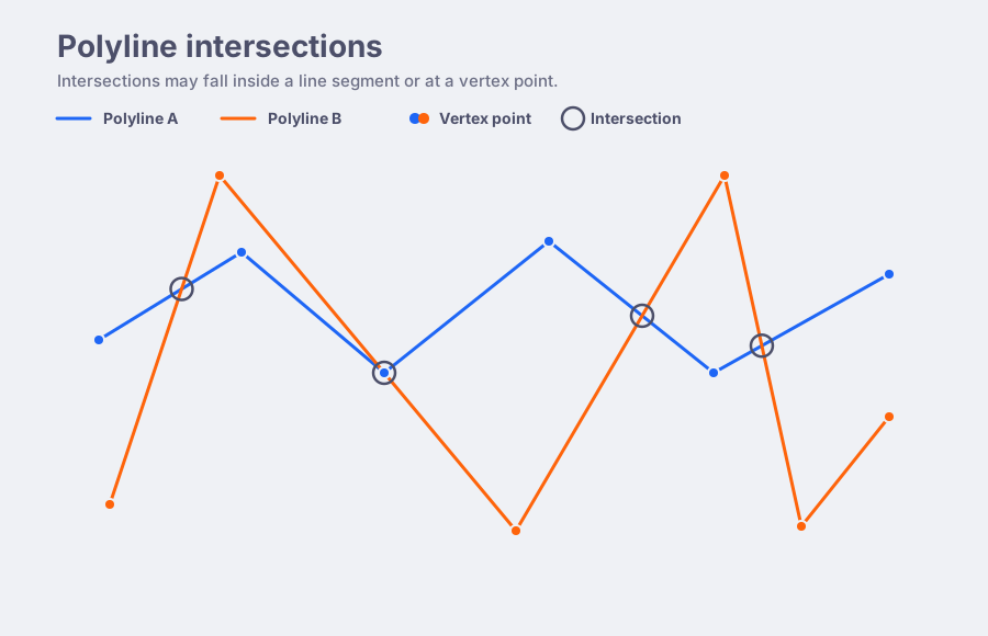
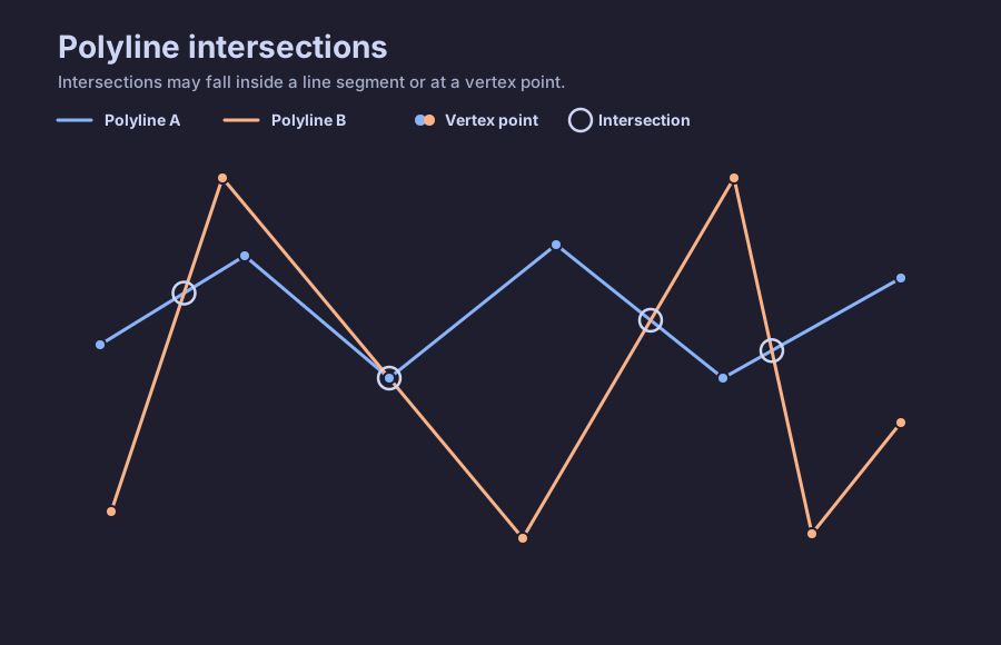
There are two things that immediately arise to be tackled but seem easy enough to deal with:

• Intersections that occur at a join point (polyline vertex) will be duplicated: we’ll find the intersection at the end of the first segment and the beginning of the next segment.
  • Solution: if another segment follows in the same polyline, we can discard an intersection at the current segment’s end, knowing we’ll find it at the next segment’s start.
• Naively, this is an O(NM) process with N and M being the number of segments in each polyline respectively. For each segment in the first polyline, we must check for an intersection with each segment in the second polyline.
  • Solution: avoid testing every segment pair by using a sweep-line algorithm or a spatial index such as an R-tree. cavalier_contours uses static_aabb2d_index to skip pairs whose bounding boxes don’t overlap.⁴ It constructs an indexed tree of axis-aligned bounding boxes by sorting a one-dimensional Hilbert curve projection.

OK, so we find all the intersections with some deduplication at the vertex points, and we’re done. But this assumes that when we discard an intersection at one segment’s end, we’ll find it at the next segment’s start. What if neither check finds it? That gives us the scenario from the introduction: an intersection at a shared point goes undetected.

Here are f64 inputs that make this happen:⁵

first_joined_start  = (-0.731982875628402, -0.00047101298950447124)
shared_vertex       = (-0.5724891158948521, 0.17395811171181397)
second_joined_end   = (-0.4895595914101475, -0.9860441419954561)
third_segment_start = (-0.35584979432021535, 0.610437944715286)
third_segment_end   = (-0.8974480982568072, -0.4807616377933941)

To see how this happens, we need to look at the parameters from the line intersection formula. Each point on a segment has a parameter from 0 at its start to 1 at its end. A strict segment test accepts an intersection only when both parameters fall within the closed range [0, 1].

The intersection calculation is a ratio of 2D cross products. For any one pairwise test, let the first segment start at p with displacement vector r, and the second start at q with displacement vector s. Each displacement vector is the segment’s end point minus its start point. The parameters t and u along their respective infinite lines are:

t = cross(q - p, s) / cross(r, s)
u = cross(q - p, r) / cross(r, s)

Here, cross(a, b) = a.x * b.y - a.y * b.x.

These formulas come from setting the two parametric lines equal and rearranging:

Let:
    L1(t) = p + t * r
    L2(u) = q + u * s

At the intersection:
    L1(t) = L2(u)
    p + t * r = q + u * s
    q - p = t * r - u * s

Taking the cross product with s:
    cross(q - p, s) = cross(t * r - u * s, s)
    cross(q - p, s) = t * cross(r, s)

Taking the cross product of both sides with s eliminates the u * s term because cross(s, s) = 0, leaving cross(q - p, s) = t * cross(r, s). Likewise, taking the cross product with r eliminates the t * r term and gives the formula for u.

The resulting (x, y) intersection point is p + t * r, equivalently q + u * s. If cross(r, s) is zero, the lines are parallel or collinear. Those cases require separate handling and are not relevant for this example.

Applying these formulas to the concrete inputs produces the following results. For the first joined segment, the parameter is:

expected: 1
computed: 1.00000000000000022

For the second joined segment, it is:

expected: 0
computed: -0.0000000000000000386165650162848455

The first result is just greater than 1, while the second is just less than 0. A strict bounds check rejects both, so the intersection goes undetected.

This is really bad: we set out to find all intersections, the intersection clearly exists, we defined the segments as sharing that exact point, and yet our code finds none.

You can find the example code here. It reproduces the floating-point miss and uses i128 integer arithmetic to verify that all three segments meet at the shared vertex.

Recovering from Disaster

There are different mitigations and solutions for dealing with this problem. One way to avoid floating-point error is to define the input geometry on a fixed integer grid⁶.

Converting the Inputs to an Integer Grid

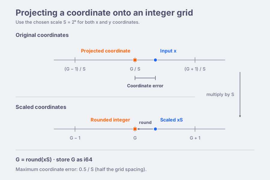
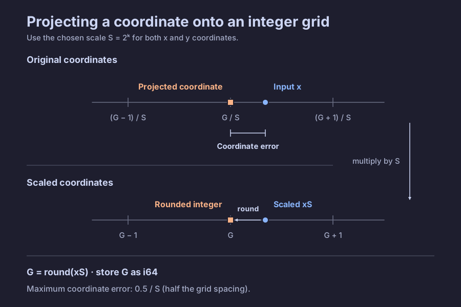
Multiply each input coordinate by a power-of-two scale S = 2^k, round to the nearest integer, and store the result as an i64. We then perform the geometric calculations with these integers. Here’s some Rust code expressing the idea:

// Input coordinates must be finite.
fn grid_scale(coords: &[f64]) -> f64 {
    let mut max_abs = 0.0;
    for coord in coords {
        if coord.abs() > max_abs {
            max_abs = coord.abs();
        }
    }

    if max_abs == 0.0 {
        return 1.0;
    }

    // We want k = min(1023, floor(61 - log2(max_abs))).
    // Evaluating log2 directly can choose too large a scale:
    // log2(16.000000000000004) can round to 4.0.
    // Read the exponent and fraction bits instead.
    let bits = max_abs.to_bits();
    let exponent = ((bits >> 52) & 0x7ff) as i32 - 1023;
    let has_fraction = bits & ((1_u64 << 52) - 1) != 0;

    // A nonzero fraction means we need a scale one power smaller.
    // The 1023 cap also handles subnormal values.
    let k = (61 - exponent - i32::from(has_fraction)).min(1023);
    2.0_f64.powi(k)
}

fn to_grid(coords: &[f64]) -> Vec<i64> {
    let scale = grid_scale(coords);
    let mut grid = Vec::new();
    for coord in coords {
        let grid_value = (coord * scale).round() as i64;
        grid.push(grid_value);
    }
    grid
}

Some things of note:

• Multiplying by a power of two changes the exponent without rounding, except when the exact product is too large or too small: abs(S * value) > f64::MAX overflows to infinity, while 0 < abs(S * value) < f64::MIN_POSITIVE may lose significant bits or round to zero.⁷ round then performs the deliberate quantization to the grid.
• We limit the scaled coordinates to [-2^61, 2^61]. As we’ll see when classifying the intersection, we need room for coordinate differences in i64 and cross products in i128, not just the coordinates themselves.
• The scale controls the trade-off between range and grid resolution. Find M, the maximum absolute coordinate across all geometry that will share the grid, then choose S = 2^k, where k = min(1023, floor(61 - log2(M))). This is the largest finite power-of-two scale that keeps M * S <= 2^61, giving grid spacing 2^-k and a supported input range of |value| <= 2^(61-k). The code reads the float’s bits to choose k rather than evaluating the logarithm in floating-point arithmetic. A larger input range lowers k and produces a coarser grid; a smaller range raises k and produces a finer grid.⁸
• An input already on the chosen grid converts without loss. Otherwise, round(value * S) / S maps it to the nearest grid coordinate, with a maximum quantization error of 0.5 * (1 / S): half the distance between adjacent grid coordinates. A smaller scale factor S puts the grid points farther apart, so rounding discards more fractional information.

Classifying the Intersection

Now that we have integers representing our coordinates, we can perform the 2D cross product arithmetic, but we need to ensure we do not overflow our fixed-size integers:

• Subtracting coordinates bounded by [-2^61, 2^61] produces a difference with magnitude at most 2^62, which fits in i64.
• Multiplying two coordinate differences produces a value with magnitude at most 2^124, so convert each difference to i128 before multiplying.
• A 2D cross product subtracts two such products and has magnitude at most 2^125, which fits in i128.

For two segments starting at p and q, with displacement vectors r and s:

D  = cross(r, s)
Nt = cross(q - p, s)
Nu = cross(q - p, r)

t = Nt / D
u = Nu / D

D, Nt, and Nu are exact integers. The parameters t and u are represented as rational numbers: a numerator paired with the common denominator D. No division is needed to classify the intersection. This is a big win: we can make the discrete decision using exact integer comparisons, without truncating a quotient or converting to floats.

if D == 0:
    parallel or collinear; not covered here
    stop

if D < 0:
    D  = -D
    Nt = -Nt
    Nu = -Nu

the segments intersect when:
    0 <= Nt <= D
    0 <= Nu <= D

The example inputs already lie on the chosen grid, so projection changes none of them. The exact joined-segment parameters are 1 and 0, while the exact parameter on the third segment is 2 / 5. Both intersections are therefore found at the shared vertex.

For the projected integer-grid geometry, this approach guarantees that an intersection at a shared vertex is not missed:

• The conversion to integer coordinates preserves the topology that the join point is shared (seg1_end = seg2_start = shared_vertex).
• The subtraction and multiplication operations introduce no error (using i128 to ensure no overflow).
• The integer coordinates support exact less-than-or-equal comparisons needed to detect and classify the intersection.

Consequences of the Integer-Grid Approach

So is this the solution to our intersection miss disaster? For the projected geometry, it prevents rounding errors from making us miss this “intersection at a shared vertex” event. But it raises more questions and problems to solve about the intersection result.

What do we return to the caller? With the floating-point approach, we assumed the arithmetic always worked and could return either the parametric t and u or the (x, y) intersection point as f64 values. With the integer-grid approach:

• We can retain the exact parameters as the rational pairs Nt / D and Nu / D because each integer fits in i128. These ratios may not be exactly representable as f64, so returning floating-point parameters can reintroduce rounding. The intersection point can have the same problem: its coordinates may lie between grid points, and converting them back to the original input scale also requires division by S.
• Fully expanding the coordinates into rational numerators can also require integers wider than i128, even though i128 is sufficient for classifying the intersection. This is because more multiplication is performed:
  • Substituting t = Nt / D into x = p.x + t * r.x gives the exact rational coordinate x = (p.x * D + Nt * r.x) / D; the same applies to y.
  • From the earlier bounds, |p.x| <= 2^61, |r.x| <= 2^62, and both |Nt| and |D| are at most 2^125.
  • Using conservative bounds, |p.x * D| <= 2^186 and |Nt * r.x| <= 2^187, giving a storage estimate of 188 magnitude bits for their sum. This exceeds the 127 available in a signed i128.

So What Did We Actually Find?

There’s a more basic problem: projecting the inputs to the integer grid can change the geometry. How does the intersection we found relate to the original f64 segments?

First consider an intersection at the exact start or end of a projected segment. Its rational parameter is exactly 0 or 1, so it can be returned exactly as 0.0 or 1.0, and we can use the original f64 segment coordinates for (x, y). Reusing the original endpoint introduces no new rounding error, but that point may differ from the projected intersection and may not be an intersection of the original f64 segments. Critically, the half-grid bound limits how much projection can move each input coordinate. It does not bound how far the intersection can move.

Ugh, how can that be? Consider two line segments that are very nearly parallel:

Let the maximum absolute coordinate from the inputs be 1, giving S = 2^61 and grid spacing Δ = 1 / S = 2^-61. Call the two f64 input segments A and B. Their start and end coordinates are:

segment    start (x, y)    end (x, y)
A          (0,  0.25Δ)     (1, 1.25Δ)
B          (0, -0.25Δ)     (1, 1.75Δ)

Scaling each coordinate by S and then rounding gives the projected integer-grid segments, A' and B':

segment    start (x, y)    end (x, y)
A'         (0, 0)          (2^61, 1)
B'         (0, 0)          (2^61, 2)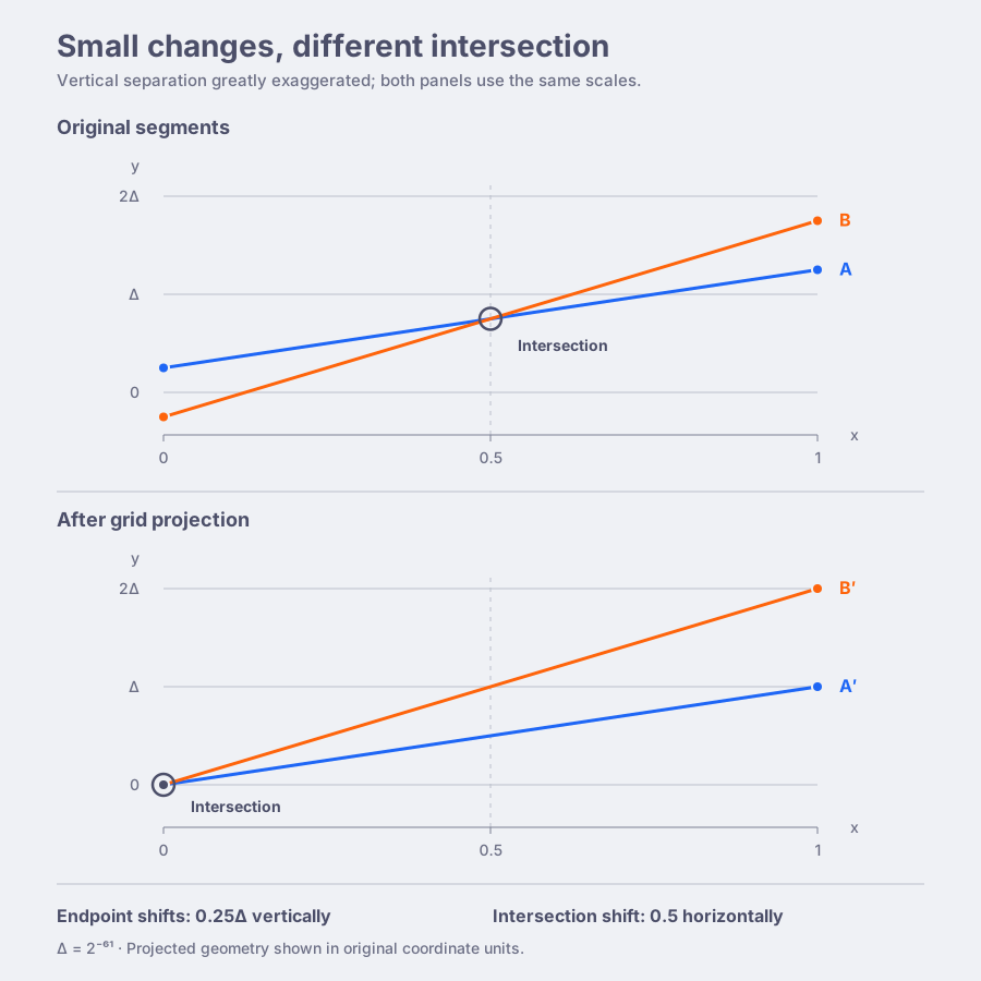

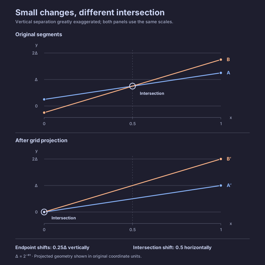
The original segments intersect at (0.5, 0.75Δ), while the projected segments intersect at their shared start. Each endpoint moved by only 0.25Δ (that’s about 0.000000000000000000108 units), yet the intersection moved half the segment length (about 0.5 units; both segments are about 1 unit long). The segments have slopes Δ and 2Δ, so their near-parallelism amplifies the small quantization error. The example repository includes this near-parallel case for reference.

This is an extreme example, but it demonstrates the subtleties involved. How we deal with nearly parallel segments depends on the application: the resulting intersection error may not matter, or it may be critical that we identify and account for it.

An intersection inside a segment gives us more questions to answer. We can’t simply reuse an endpoint. We can retain t as the exact rational pair Nt / D, but what if the caller needs an f64 or an (x, y) point?

Converting the rational parameter to f64 before calculating the intersection point avoids the large integer products, but reintroduces rounding error. Keeping the coordinates exact can require wider integers: i128 was enough to decide that the segments intersect, but may not be enough to represent the intersection point exactly. We now have both the error from projecting the inputs and any error from approximating the output to account for.

The key advantage here is that integer projection preserves the specific topological relation we started with: seg1_end = seg2_start = shared_vertex. Exact integer arithmetic then lets us test intersections in the projected geometry without rounding errors contradicting our mathematical reasoning.

But that guarantee applies to the projected geometry. As the nearly parallel example shows, even small changes to the inputs can produce a very different intersection. Preserving the join doesn’t tell us how that intersection relates to the original geometry.

What’s next?

There’s more to explore with this solution, but in part 2 I’ll look at other approaches and some of their implications.